
A scale-free network is a network with self-similar structure. As you zoom in on parts of the network, the sub-network resembles the overall network. In this way, scale-free networks are the network analogy of fractals. (Read previous posts about fractals, or fractals in nature.) Fractals arise in many natural systems like coastlines, snowflakes, and topology; likewise many naturally arising networks are self-similar. Examples include links on the internet, social networks, and protein interaction networks. Understanding the structure of a network helps us to understand the types of behavior that can occur on the network. Some network structures are more prone to failure or instability, or different types of failure or instability.
Scale-free networks have a sort of hub arrangement. Some elements connect to a bunch of other elements, while most connect to just a few. Going back to the social network analogy, the hubs are those people with 1500 friends on Facebook, while most people have 100 or so. In the picture below, a random network is shown on the left, and a scale-free network is shown on the right (hubs shown in grey). In the random network, all the elements have roughly the same number of connections, with some slightly more, some slightly less. The scale-free there has more variation in number of connections amongst elements.

From Wikipedia page on scale-free networks.
Getting more mathematical, the number of connections an element has gives its degree. An element with 3 connections has a degree of 3. We can say, hypothetically, that element 1 has a degree of 2, element 2 has a degree of 6, element 3 has a degree of 2, etc. We have degrees for all of the elements of the network. If we organize this set of degrees into a histogram (where we bin by degree value– in our example, we had counted two of degree 2, and one of degree 6) we get a degree distribution.
If something is distributed normally, the histogram has a bell-shape to it, like the first picture below. If you did a histogram of the height of all the people in your city, it would be a normal distribution. If it is distributed in a scale-free fashion, there are a few high value elements (high degree in our case), and a lot of low value elements. This gives the bottom picture, with a peak at a low value and a long tail into the higher values. The wealth distribution in your city probably looks like the scale-free distribution. If you take the log of the values on the scale-free distribution, you will get a straight line. This is because the logarithm is the inverse of the function 10^x; if you take the log of something, you can see its behavior on the 10^x scale, which gives you insight into how it behaves across multiple powers of 10, or its “scaling free” behavior.

From Wikipedia article on normal distribution
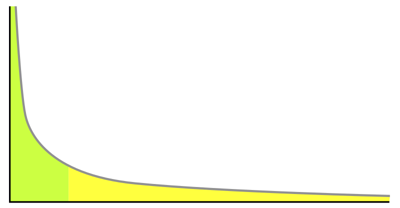
From Wikipedia article on power-law distribution
If you are interested in other basic explanations of more advanced science, also check out my posts on synchrony, chaos, network theory, and small-world networks.


