
Please excuse my inconsistent posting of late, I have been deep down the rabbit hole of science. Last week, I attended the Society of Industrial and Applied Math (SIAM) dynamical systems conference. What fun!
I learned about Turing Patterns, named for mathematician Alan Turing. Complex patterns can arise from the balance between the diffusion of chemicals and the reaction of those chemicals. For this reason, Turing’s model is also called the Reaction-Diffusion model. In general, these kinds of patterns can arise when there’s some kind of competition.
This sounds abstract, but suspected examples in nature abound. Have you ever wondered how the leopard got his spots or what’s behind the patterns on seashells? We often don’t know the chemical mechanisms that produce the patterns, but we can mathematically reproduce them with generic models.

Image from wired.com discussion of Turing patterns.
Mary Silber and her grad student Karna Gowda presented research on Turing patterns in the vegetation of arid regions. When there isn’t enough precipitation to support uniform vegetation, what vegetation will you observe? If there’s too little water, their model yields a vegetation-free desert. Between “not enough” and “plenty” the model generates patterns, from spots to labyrinths to gaps. Their work expands at least two decades worth of study of Turing patterns in vegetation.
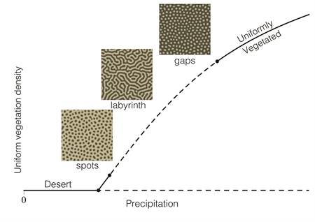
Figure by Karna Gowda, see the full article at SIAM news.
Silber and Gowda considered an area in the Horn of Africa (the bit that juts east below the Middle East). Here, stable patterns in the vegetation have been documented since the 1950s. They wanted to know how the patterns have changed with time. Have the wavelengths between vegetation bands changed? Are there signs of distress due to climate change? By comparing pictures taken by the RAF in the 1950s to recent satellite images, they found that the pattern were remarkably stable. The bands slowly travelled uphill, but they had the same wavelength and the same pattern. They only observed damage in areas with lots of new roads.
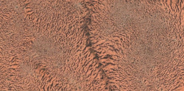
From google maps of the Horn of Africa! I screen-capped this from here.
Turing patterns have even been studied experimentally in zebrafish. Zebrafish stripes might appear stationary, but they will slowly change in response to perturbations. So scientists did just. Below is a figure from the paper. The left shows the pattern on the zebrafish, the right shows the predictions of the model.
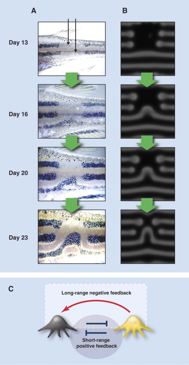
Experimental perturbations to the patterns of zebrafish are well-predicted by the Turing model. Read more in this excellent Science paper.
The model has been used to explain the distribution of feather buds in chicks and hair follicles in mice. Turing’s equations have even been used to explain how fingers form.
If you want to learn more, the links above are a great start. And if you want to play with the patterns yourself, check out this super fun interactive. These waves aren’t stationary like the Turing patterns I described here, but they arise from similar mathematics. The interactive can make your computer work, fyi.
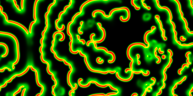
Reaction-diffusion pattern I generated with this online interactive. It’s super fun!

